Intuitively, neural networks with billions or trillions of parameters should not be able to generalize, they should catastrophically overfit the training data. But deep neural networks have demonstrated remarkable generalization abilities for a variety of tasks.

Why is that?

The cleanest mathematical story that explains it is called Singular Learning Theory. SLT might end up being a key mathematical tool for AI safety and interpretability in the future.

What is SLT and what problem is it solving? And what does it have to do with ice?

The problem

Neural networks cannot be analyzed with statistical tools that work well for classical models like linear regression or logistic regression. Why not? Like many of us, they have degeneracies. In classical models, the loss landscape has curvature everywhere, the Fisher information matrix is full rank. With less jargon: wiggle any parameters and your loss smoothly changes. You can try it yourself on this simple, two-parameter linear regression toy model.

Small changes in the parameters change the loss gradually on the surface of a smooth bowl. That’s not true for neural networks. Some neurons may have zero outgoing weights and the order of neurons within a layer doesn’t change the model. The loss might not respond to wiggles of all parameters. This makes the model singular.

In a classical model, all parameters are “effective” because they all affect the model’s function. The model’s complexity can be characterized by the number of these parameters, $d$. This number shows up in many places: Bayes free energy, BIC penalty, posterior entropy and so on. (Usually $d$ is divided by two. The factor of $1/2$ is a math artifact that falls out of the $d$-dimensional Gaussian. The conventional complexity metric is $d/2$.)

Neural networks are different: because of their degeneracies, the number of effective parameters is usually much lower than $d$. (Consequently, a typical neural network has a smaller effective complexity than $d/2$.) These degeneracies are the secret to why they actually generalize so well.

How so?

What is Singular Learning Theory?

SLT is a branch of statistics developed by Sumio Watanabe. It is the mathematical machinery that lets us analyze models whose parameter space is not one-to-one with the function they represent. Put differently, where the model is not a smooth bowl. Like a neural network.

The math, centered around algebraic geometry, is complicated, but the headline result, $\lambda$, is easy to understand. $\lambda$ denotes real log canonical threshold (RLCT), which replaces $d/2$ in singular models as a measure of complexity. The theory is compatible with regular models, so for these $\lambda = d/2$.

For any model, RLCT measures how much of the parameter space sits near minimum loss. If that makes no sense, you might find the hill-climbing metaphor of gradient descent useful here. Picture that you are sitting at some low loss point on the loss landscape and look around yourself. Can you wander around without starting a steep climb back up? Are you in a fjord or vale? RLCT measures this. In practice, $\hat{\lambda}$, the local version of RLCT is calculated, which measures the shape of the loss landscape around a specific point. It is also called local learning coefficient (LLC).

Put simply, low LLC around a point means you can walk around without much climbing, while high LLC means the loss will quickly increase as you leave the point in the parameter space.

Some natural basins with different shapes. Top: Black Canyon of the Gunnison, Colorado (CC BY-SA 4.0 Terry Foote). In this 2D loss-surface metaphor the model is brittle, small steps away from the local minimum force you up a steep cliff. Bottom: Death Valley, California (Public Domain, National Parks Gallery). An analogy for a degenerate, robust model where you can wiggle parameters without big changes in the loss.

How is LLC useful?

Here’s a surprising math fact: neural networks learn like ice melts¹.

When water is frozen, the water molecules sit in a crystal structure and have a limited number of valid ways to be arranged. The number of possible microstates, that is, the entropy, is relatively low. As the temperature rises, two competing pressures of energy (favoring ordered arrangements) and entropy (favoring disorder) shift their relative importance and, above $0^\circ\text{C}$, energy loses the tug of war: a phase transition happens. The entropy surges, because there are more possible molecule arrangements when the ice crystals loosen.

In the beginning of neural network training, the parameters can be in many different configurations at similar loss. Entropy is high. As the training progresses and the model starts to fit the data, the loss drops and so does the entropy: just like ice, the structure of the network becomes more ordered, at least initially.

Here’s what’s interesting: sometimes, well after the loss converges, the entropy starts climbing. The network drifts into a region of the parameter space where many different parameter configurations produce similar loss due to the degeneracies of the model. The ice melts. The model’s representation of the training data becomes less brittle, more stable. This often corresponds to better test set accuracy and a simpler representation of the training data. Later we will see a hands-on example.

Similarly to how entropy describes the multiplicity of microstates in physical systems, LLC characterizes the multiplicity of microstates at the current low-loss point in the parameter space. Its change over the training can indicate qualitative changes in the network’s weights. Indeed, Watanabe’s math predicts that neural networks go through similar phase transitions as physical systems. SLT’s free energy is the same mathematical object that describes phase transitions in thermodynamics and statistical mechanics.

Here’s the most important sentence of this post: The model is naturally drawn towards simpler representations of the data, because those representations occupy a larger volume in the parameter space. Occam’s razor isn’t an externally imposed preference, it falls out of the math.

LLC measures qualitative jumps between regions in the loss landscape, something that is not visible from just the loss curve. A drop in LLC during training means that the model has arrived at a simpler, more stable representation of the training data. A concept “clicked”. The model generalized.

This matters for AI safety. Proponents of developmental interpretability (devinterp) believe that LLC can help us track when new abilities are acquired during training and how strongly they are established in the model. It may also help us detect when AI models try to game safety mechanisms.

How is LLC calculated?

Here’s the bad news: calculating the exact value of LLC is intractable for even relatively small neural networks. It involves a process from algebraic geometry called resolution of singularities applied to the loss landscape’s structure. The upper-bound time complexity is roughly $O\left(\mathrm{Ackermann}(d)\right)$ or $O\Bigl(\underbrace{2^{2^{\cdot^{\cdot^{\cdot^{2}}}}}}_{d\ \text{twos}}\Bigr)$. Please come up with your own popular science intractability analogy here (atoms in the Universe, seconds since the Big Bang, yada yada).

If you can’t evaluate an integral analytically, the next best thing is to rewrite it as an expectation and estimate it by sampling. How to do the sampling? The answer is good old gradient descent with a twist: added noise. Stochastic Gradient Langevin Dynamics (SGLD) works just like the standard optimizer step, but it adds some Gaussian noise to each parameter. In our hill climbing analogy: you randomly wander around a specific point to get a feel for the shape of the landscape. The gradient keeps you near the low-loss region but the random noise pushes you to explore.

As you “walk around”, you collect loss samples from trajectories around the area. You can try it yourself below.

The difference between these samples and your original loss gives you an idea of the shape of your valley: wide and flat or steep and V-shaped. LLC is the scaled average of these differences and captures the shape in a single number.

Here $\overline{L}_{\text{SGLD}}$ is the mean loss over SGLD samples. The denominator is the effective temperature where $\eta$ is the learning rate and $\varepsilon$ is the noise scale.

The formula for wandering around (SGLD) is as follows:

The first part looks like a gradient descent step on a tempered, regularized loss. The second part is the Gaussian noise. $\epsilon$ is the step size, $n$ is the dataset size, $\gamma$ is the localization strength, $\sigma$ is the noise strength. $\beta$ here means the inverse temperature which is $1/\log n$ for Watanabe’s standard estimator.

The optimal hyperparameters are subject of active research. In the toy examples below I use the standard estimator with $\gamma = 1.0$, $\sigma = 1$, and $\epsilon = \sqrt{2\eta}$ where $\eta$ is the learning rate. Each LLC estimate uses 5000 SGLD steps with the first 1000 discarded as burn-in.

Toy models

I used the following simple experiments to develop my own intuitions on local learning coefficient (LLC) and Stochastic Gradient Langevin Dynamics (SGLD). First, we’ll look at a regular model and estimate its complexity. Then we’ll move on with a simple neural model with degeneracies. Finally, we’ll look at LLC evolution over the training. The notebook is available here.

Warm-up: Linear Regression (2 parameters)

A simple linear model $f(x) = wx + b$ trained on the dataset $y = 3x + 2$. The loss landscape is a convex bowl with a single minimum at $(w, b) = (3, 2)$. This is a regular model so we expect the LLC to approximately match $d/2$, that is, 1. We train the model for some steps, visualize the landscape, and run SGLD from the trained weights to get a rough LLC estimate.

# DATASET: Linear Regression (y = 3x + 2)
X = torch.linspace(-1, 1, 100).reshape(-1, 1)
Y = 3 * X + 2

# MODEL: 2 parameters (weight and bias)
model = nn.Linear(1, 1)

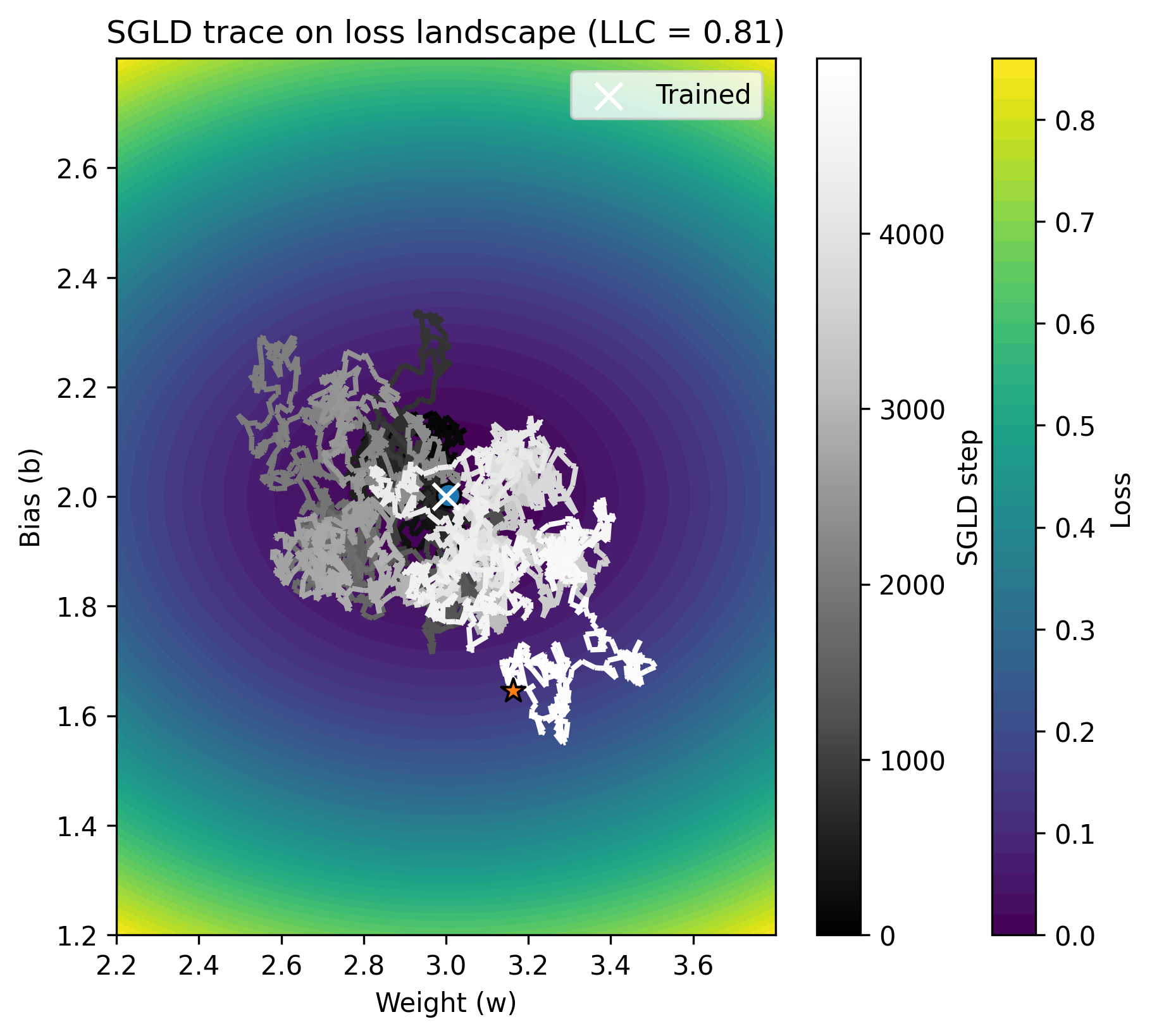
The plot below shows the loss landscape, the parameters after training near the minimum, and the trajectory the SGLD took (the circle marks the start, the star marks the end). The LLC it calculated is $\approx 0.81$, which is not too far from what we expect from a two-parameter regular model: $d/2 = 2/2 = 1$. The trajectory’s differences from base loss look like [-0.02838482 -0.02812932 -0.03070474 ... 0.0922314 0.08985042 0.09166867]. Their scaled average gives the estimated LLC. The scaling factor $n\beta = 100 \cdot \frac{1}{\ln 100} \approx 21.7147$ for the data set of 100 elements.

You can see how the chain explores the bowl without straying too far from its center. In practice, for more statistical stability, several chains (independent trajectories) are used to estimate LLC, but in this toy model we only run one.

Nonlinear Model: Single Hidden Neuron (4 parameters)

Here’s a more interesting case. A tiny MLP with one hidden neuron and tanh activation:

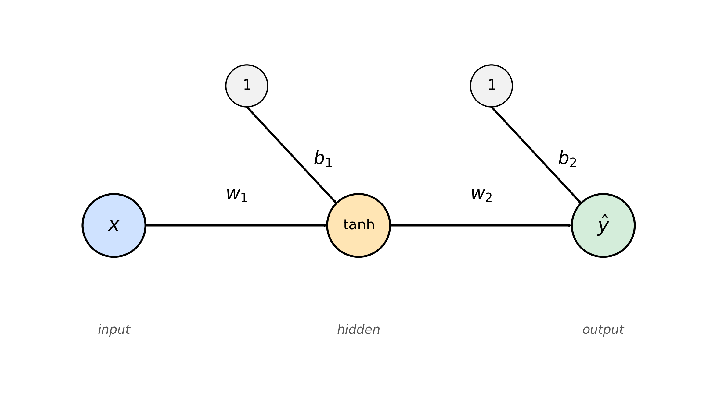
This has 4 learnable parameters $(w_1, b_1, w_2, b_2)$. Unlike the linear case, the loss landscape is non-convex and has symmetries (e.g., flipping the sign of $w_1$ and $w_2$ simultaneously gives the same function).

In the notebook I provide several toy datasets that you can play with. Below I’ll use $y = \sin(3x) + 0.3x$

# DATASET: Sinus plus trend (y = sin(3x) + 0.3x)
X = torch.linspace(-2, 2, n).reshape(-1, 1)
Y = torch.sin(3 * X) + 0.3 * X

# NONLINEAR MODEL: 1 hidden neuron => 4 parameters
class TinyMLP1(nn.Module):
    def __init__(self, activation="tanh"):
        super().__init__()
        self.fc1 = nn.Linear(1, 1)   # w1, b1
        self.fc2 = nn.Linear(1, 1)   # w2, b2
        self.act = torch.tanh

    def forward(self, x):
        h = self.act(self.fc1(x))
        yhat = self.fc2(h)
        return yhat

model = TinyMLP1()

Since the model has 4 parameters, there are $\binom{4}{2} = 6$ distinct 2D slices through the loss landscape. Viewing them all at once reveals which parameter pairs the sampler explores freely due to its degeneracies and where it stays tightly concentrated.

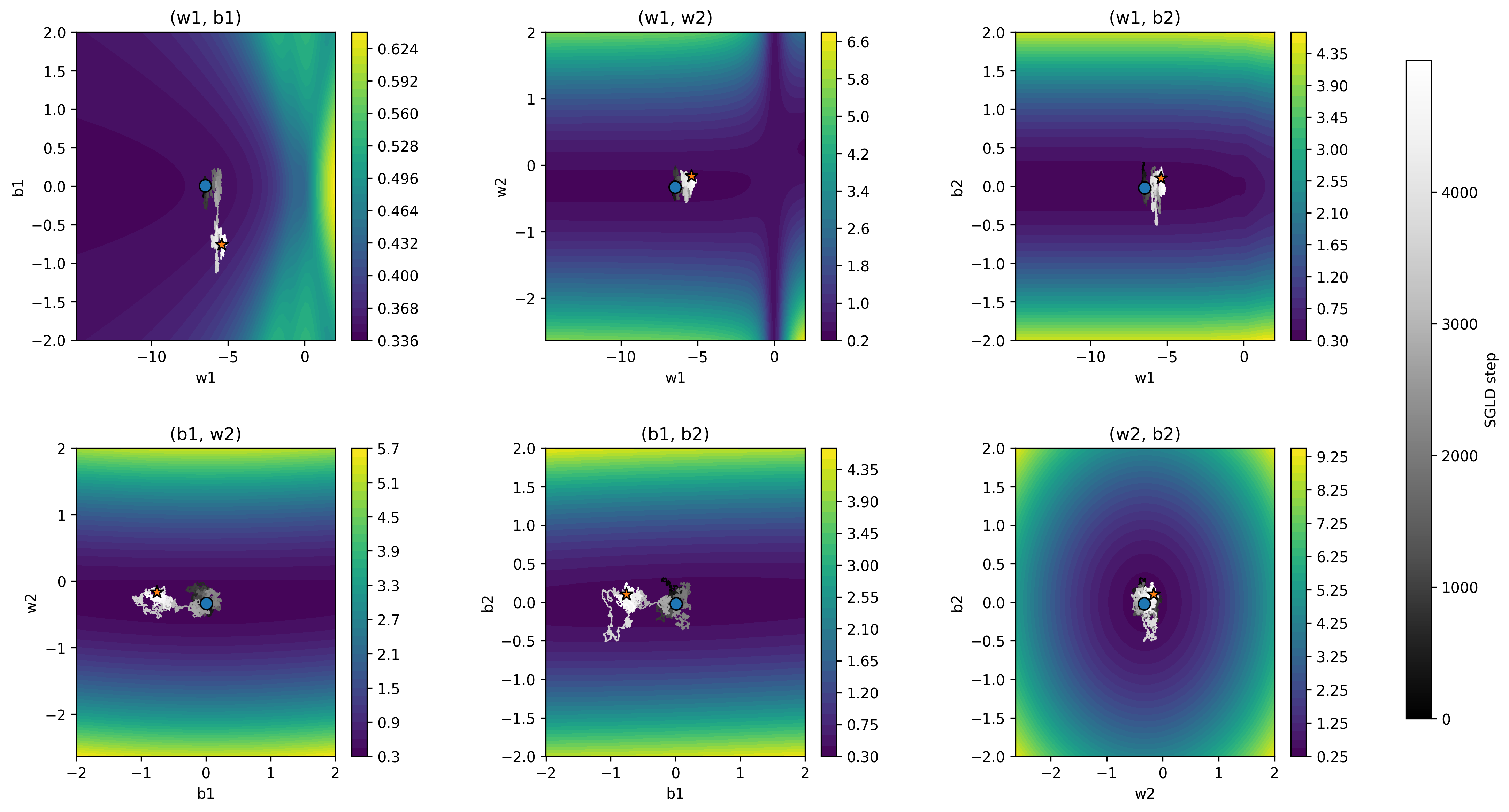
The estimated LLC is 0.7178. But remember, the sampling is stochastic due to the noise. To get more reliable estimates it’s standard practice to run several chains, each starting from the trained checkpoint weights. The chart below shows 4 chains using different colors.

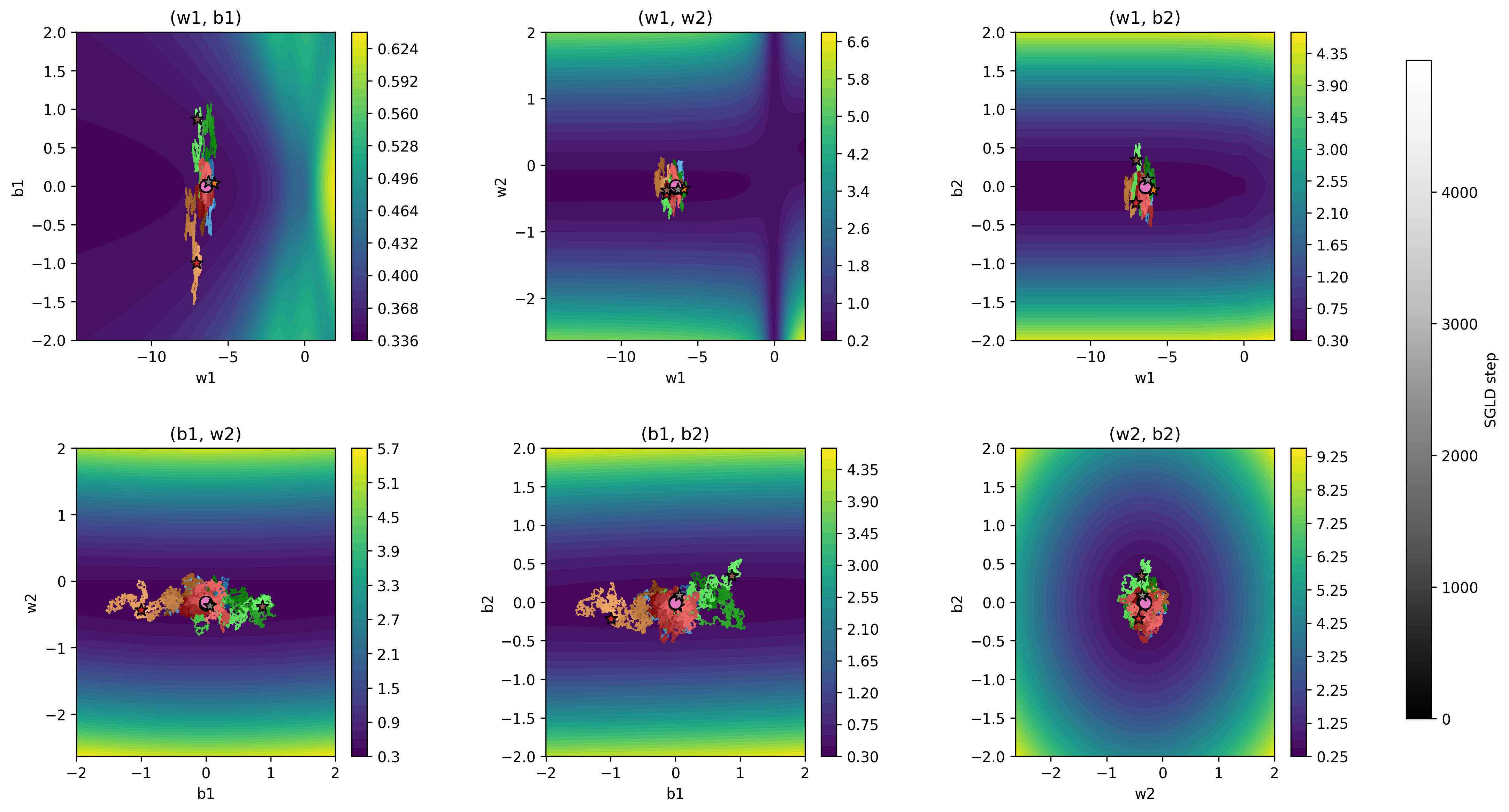
The averaged estimated LLC is 1.0962 ± 0.2530. It sits comfortably below $d/2$ indicating a smaller number of effective parameters compared to a regular model with the same number of parameters, as we expected.

LLC Over Training: The “dev” in devinterp

Developmental interpretability (“devinterp”) analyzes the capabilities of models as they go through training. Some basic capabilities tend to emerge sooner, while more complex ones “click” later in the process. As discussed above, LLC estimation is a useful tool to analyze whether a model, or a subset of its parameters have arrived at a simpler, stable representation of the training data.

We can estimate LLC at given training checkpoints. As the model learns, the local geometry of the loss landscape changes and so does $\hat\lambda$.

Below, we train a fresh model from scratch, saving checkpoints at regular intervals. At each checkpoint we run SGLD and estimate the LLC. We then plot:

1. LLC vs training step the developmental trajectory of model complexity
2. SGLD traces at selected checkpoints showing how the sampler explores different geometries at different stages of training (projected onto the $(w_1, b_1)$ plane)

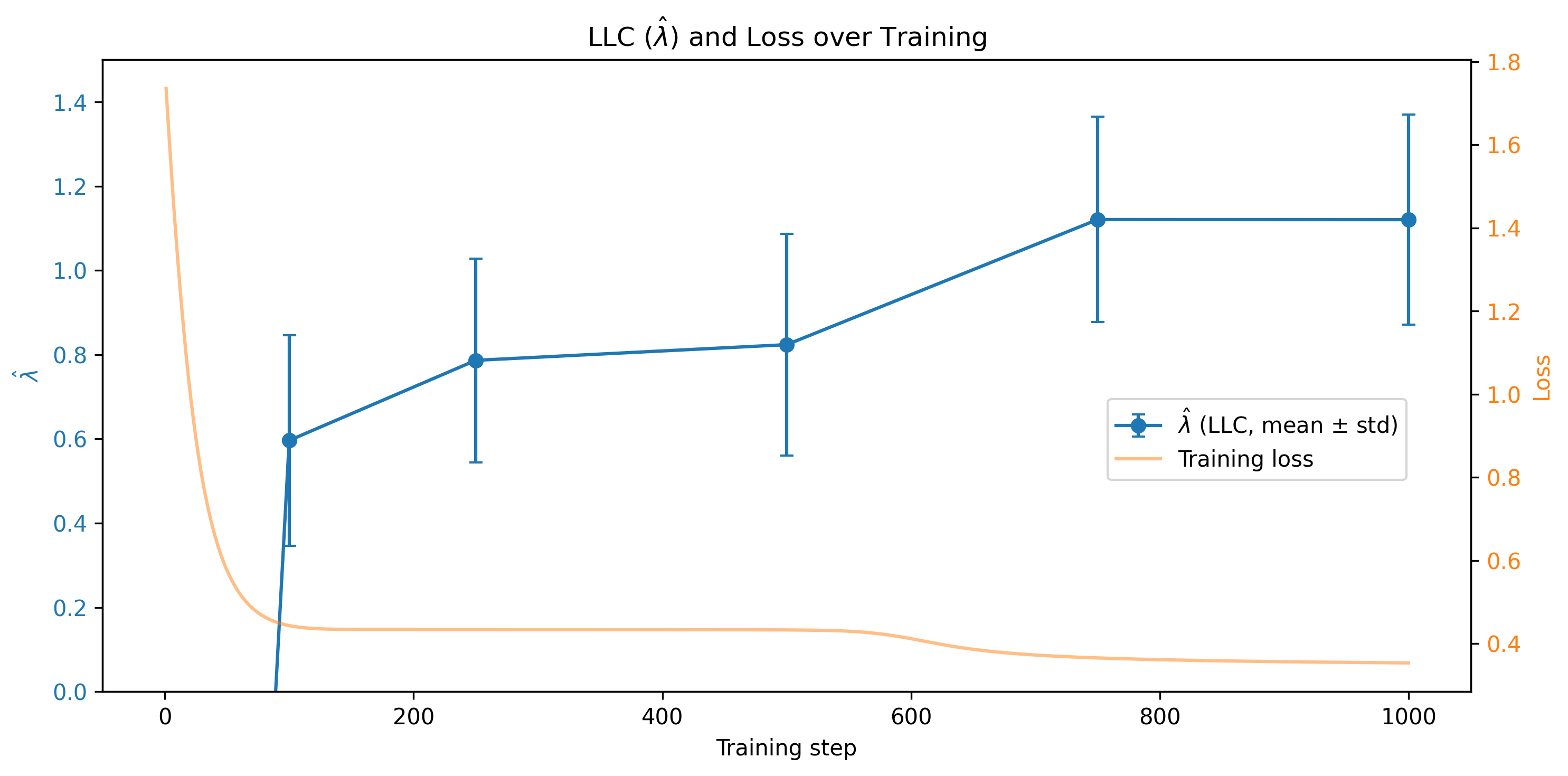
At step 0 the LLC can get negative as the model is completely untrained and SGLD steps may actually improve the loss. There is a sharp drop in the loss between step 500 and 750 with a corresponding surge in LLC. This is a state transition that indicates a move toward a somewhat higher complexity model, although it’s an overstatement for a very simple toy MLP like this one. We see no ice melting or grokking here, the data and the model are too simple.

Grokking and state transitions

If we want to see meaningful state transitions, we need a bigger model. What happens if we throw a heavily over-parameterized model on a simple, 1,000-item bit parity dataset?

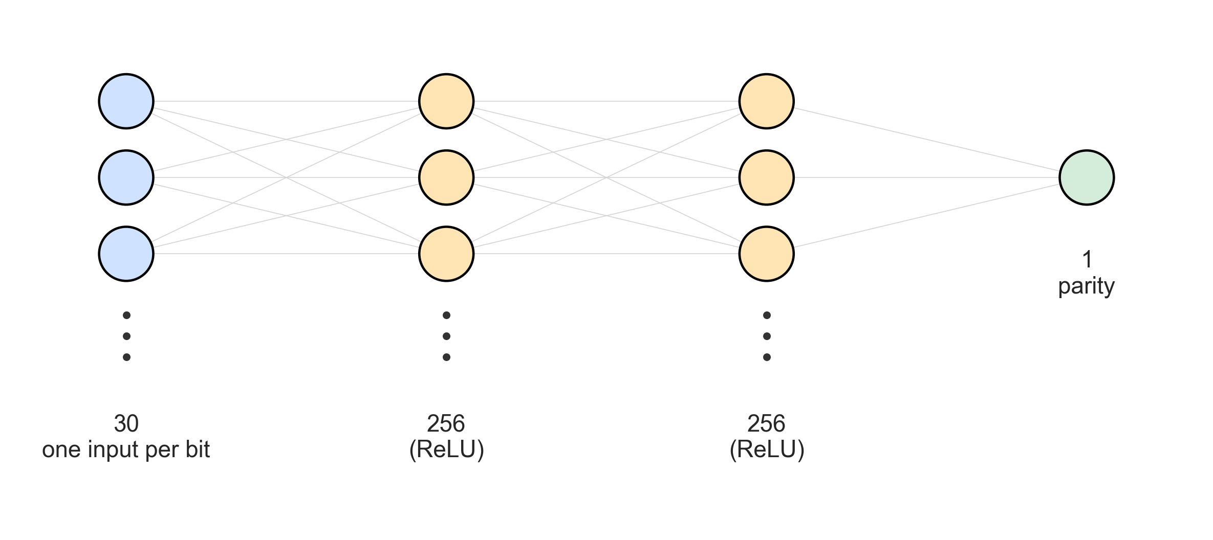
In this example (notebook here) we set up a network with $30 \to 256 \to 256 \to 1$ neurons with ReLU giving us ~74k parameters. We are still nowhere near commercial-sized models, let alone SOTA foundation models, of course, but this is a huge overkill for a simple dataset of this size.

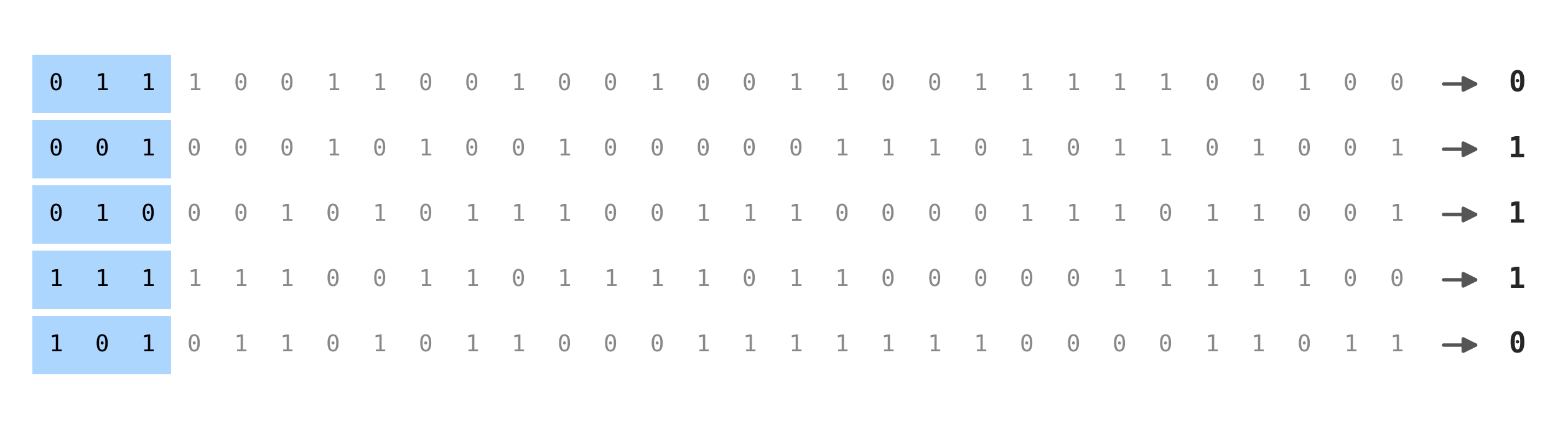
# DATASET: parity (XOR) of the first K bits on random binary numbers of N_BITS length
N_BITS = 30
K = 3
X = torch.randint(0, 2, (n_samples, N_BITS)).float() * 2 - 1
parity = (X[:, :K] < 0).sum(dim=1) % 2
Y = parity.float().unsqueeze(1)

# MODEL: 2 hidden layers of 256 neurons each => 73,985 parameters
class MLP(nn.Module):
    def __init__(self, width=256):
        super().__init__()
        self.net = nn.Sequential(
            nn.Linear(N_BITS, width), nn.ReLU(),
            nn.Linear(width, width), nn.ReLU(),
            nn.Linear(width, 1),
        )

    def forward(self, x):
        return self.net(x)
        
# OPTIMIZER: The toy models above used simple SGD, here we "graduate" to AdamW with weight decay so that the model does not stay stuck at the memorized solutions. 
opt = optim.AdamW(model.parameters(), lr=1e-3, weight_decay=5e-2)

The training evolution chart below shows how the model first memorizes the training set. This is expected because of the small data set and comparably big model that is able to simply remember the correct answers. The training set accuracy quickly jumps to 100%. On the test set, the data the model has not seen, the model does around as well as flipping a coin. LLC remains flat until step 7,500, then something interesting happens. Weight decay pushes the model around in the loss landscape until there’s a “click” and the model settles for a simpler, more general solution. LLC drops sharply from ~420 to ~150. The test set accuracy rises to 100%.

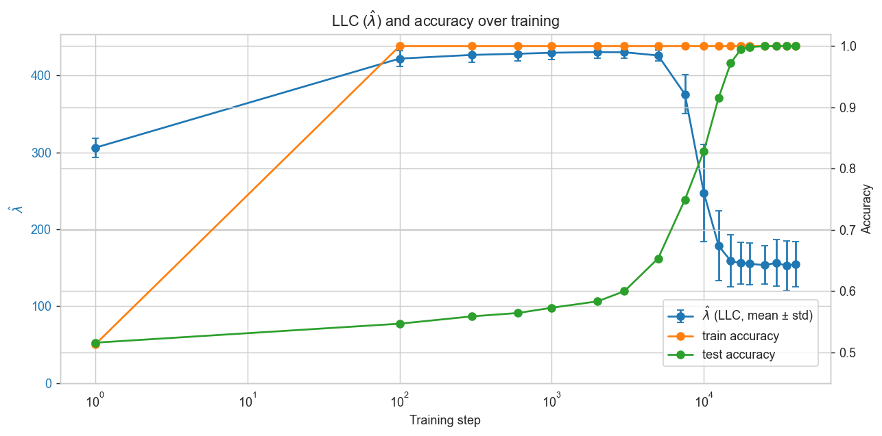
This is the phase transition predicted by Watanabe’s math: the “melting” moment in our ice analogy. Suddenly, the model’s configuration changes, the number of effective parameters drops and the multiplicity of valid states increases dramatically. The water crystals break loose, liquid water allows significantly more freedom in how molecules are arranged.

The LLC drop indicates something that loss itself cannot: the model has arrived at a simpler, more degenerate representation of the problem. The model has stabilized and generalized.

SLT on bigger models

By now you might be asking: can we do LLC estimation on really large models, like SOTA foundation models?

Yes, we can, and that’s the point. If we hope to use SLT in the future to understand how large language models or world models understand concepts, how they generalize and how strongly they grasped concepts, we need to apply the above on models with billions or trillions of parameters.

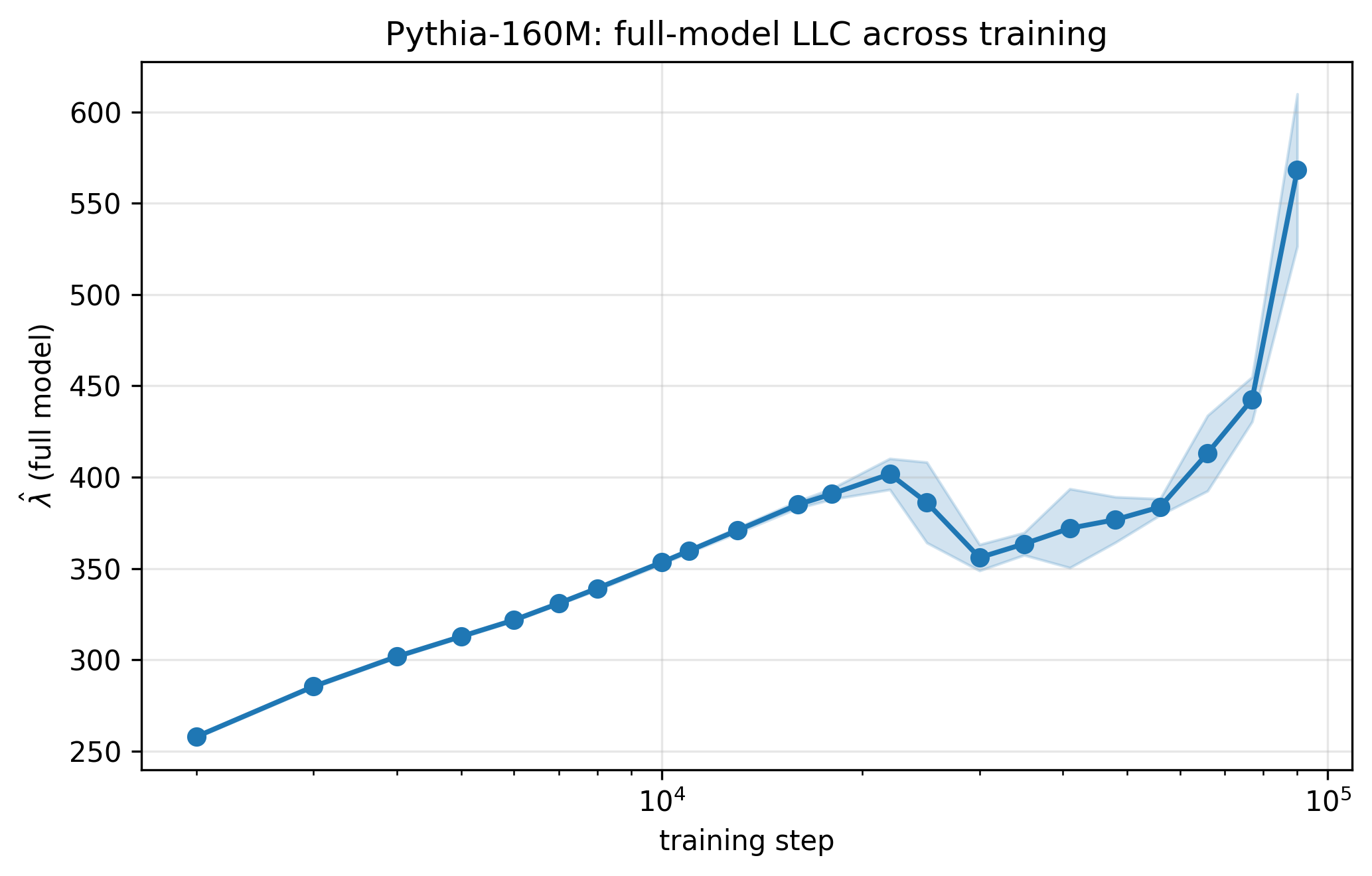
The Pythia model family by EleutherAI was expressly created to help research into how LLMs learn. The model architecture, training data, as well as training checkpoints are public. The estimated LLC evolution on the 160M parameter model looks like this:²

See the notebook here.

LLC monotonically grows then drops and goes back up. This is not the full training and by itself does not tell us much. The model can go through shifts in effective complexity during the training. But this is just the bird’s eye view. When estimating LLC, we don’t always have to consider all the parameters. Arbitrary subsets of parameters can be examined separately. This technique is called restricted LLC.

This model has 12 hidden layers and we can estimate LLC for each separately. Something interesting happens here.

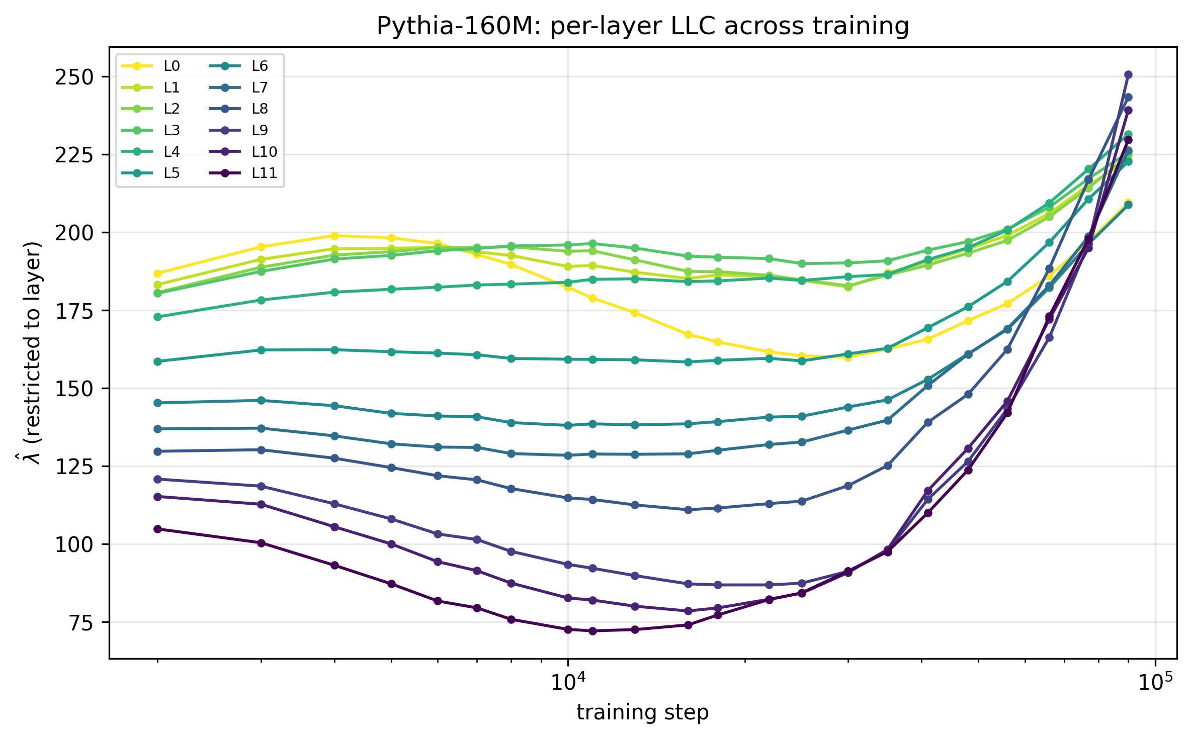
Early in the training, complexity is front-heavy, the first layers carry much more of it, almost perfectly ordered by estimated LLC. As the training progresses, the complexity starts to bubble up to deeper layers.

One way to interpret this is that in a deep neural network, the early layers generally extract lower level features: low-order statistics, frequencies, simple correlations. Before these are baked in and are sufficiently generalized, later layers can’t build on them. Once the early representations are stable and shed some of their complexity, later layers can start extracting higher level patterns and increase in effective complexity.

Layer-wise analysis is just one way to do restricted LLC. Attention heads, individual FC layers and just about any subset of weights can be independently analyzed, often combined with a restricted training data set or curriculum training.

This is the kind of developmental interpretability analysis that makes SLT a powerful tool for AI safety research. SLT may help us catch capabilities the moment they emerge during training, characterize how well the model generalizes, how strongly model fine-tuning have changed internal concepts, and even perhaps detect faking alignment.

Further reading

I hope that this blog-post caused a state transition in your brain, and you’ve by now grokked the basics of SLT on neural networks. Please know that a simple post using a lot of layman wording cannot do justice to Singular Learning Theory, but I hope it succeeded in piquing your interest. If so I recommend continuing from here:

• Sumio Watanabe’s homepage on SLT
• Wei, Murfet, Gong, Li, Gell-Redman & Quella 2022, “Deep Learning is Singular, and That’s Good”
• Jesse Hoogland’s posts on LessWrong
• Timaeus, the research organization working on SLT and AI safety
• Jesse Hoogland’s talk on SLT
• Stan van Wingerden’s talk on SLT
• Devinterp Python library