What language do language models speak?

July 22, 2026

Has this ever happened to you?

You are talking to someone in a non-native language, say English, and your eyes glance over some text written in your mother tongue. You unconsciously flip the switch and start speaking in your native language to your friend’s surprise.

Can we trip up language models similarly? What’s the “mother tongue” of LLMs anyway? Can we make them forget how to speak a language? And can we use the same trick to unrestrict language models and have them write explicit erotic fiction of tech CEOs?

Do Androids Dream of Electric Sheep in English?

Modern LLMs are multilingual but their training data is overwhelmingly in English. For example, only about 8% of Llama 3’s pretraining tokens were non-English. The training data of commercial models is a closely guarded secret, but it’s likely that they are overwhelmingly English-biased simply because text on the internet is overwhelmingly in English.

Yet these models speak multiple languages and they do well on multilingual tasks. When you ask a question in Japanese, do they “think” in Japanese?

It’s been theorized that they don’t. Instead, they first translate the question to some English-flavored concept space, they think there, then translate the answer back to Japanese. Wu et al. (2024) borrowed a term from neuroscience for this shared concept space: semantic hub. They and others provided evidence for its existence using logit lenses.

Reading the model’s mind

Large language models generate text roughly like this:

1. Each token in the prompt is one-hot encoded to a vector the size of the vocabulary.
2. These vectors are then projected into a smaller dimensional vector space. The projection is learned during training and it’s called embedding.
3. The smaller dimensional vectors are then passed on to the first layer where some learned math is performed on them, changing their values. This learned math lets them exchange information and pick up relevant knowledge stored in the model’s weights.
4. They are then passed on to the next layer, which does its own learned math and passes it on. The passed on vectors between layers are called residual stream.
5. After the last layer, the last vector gets “unembedded” using another learned projection (the unembedding matrix). The result is a vector the size of the original one-hot encoding, but this time it contains non-zero values at most, if not all, positions (the logits).
6. These values are softmaxed, converting these values to probability scores for each token. The generated token is chosen from the top probability tokens.
7. The new token gets appended to the original prompt, then rinse and repeat.

The idea behind logit lenses is the observation that residual streams contain semantically relevant information already before the last layer. The process resembles drafting and progressively refining a concept across the layers. Logit lenses simply apply the unembedding matrix prematurely after each layer (instead of just the last one) so that in-between logits can be observed and interpreted.

Fourteen questions in five languages

A simple experiment to find the semantic hub could look like this: the model (the 42-layer Gemma 2 9B in this case) is asked a simple question in multiple languages. The logit lens reveals a similarity in the residual stream of forward passes in different languages. The prompts consist of fill-the-gap questions like the ones below. The test was done with 14 different questions making sure the answers don’t have overlapping tokens and that the model is competent at coming up with the correct answer.

Language	Prompt	Answer
English	The bright star that gives the Earth light and warmth. It is called	sun
Spanish	La estrella brillante que da luz y calor a la Tierra. Se llama	sol
Hungarian	Az égen ragyogó csillag, amely meleget és fényt ad. A neve	nap
Japanese	空に輝き、昼間に光と熱を与える星。これは	太陽
Chinese	在天空照耀、给白天带来光和热的星球。这叫	太阳
English	The red liquid that flows through your veins. It is called	blood

The chart below shows the probability the model assigned to the answer token in English (e.g. sun) versus the answer in the prompt’s native language (e.g. 太陽).

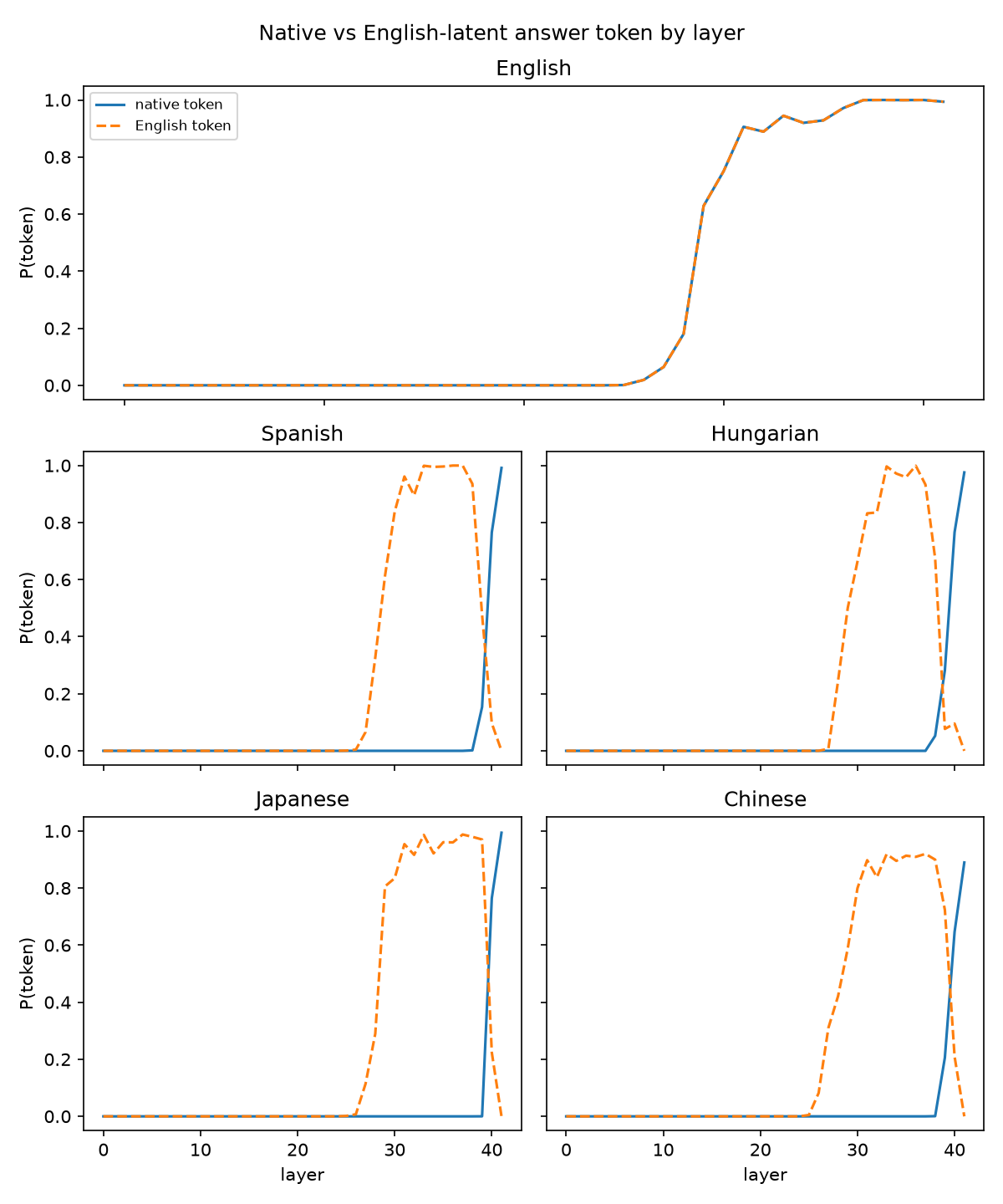
Of course, the English token is the native token on the first panel, so their probabilities are one and the same. But notice how the probability of the English token rises before the native token for non-English languages, peaking somewhere around layer 22-23 then collapsing and giving way to the native answer. The model comes up with the English response first, just to “translate” it back to the prompt’s language in the last layers.

The average English token probabilities across all 14 questions cross above 0.5 in all cases. Does this really confirm the English semantic hub? We can get a stronger signal by checking whether the correct English answer token is the most likely token at each layer.

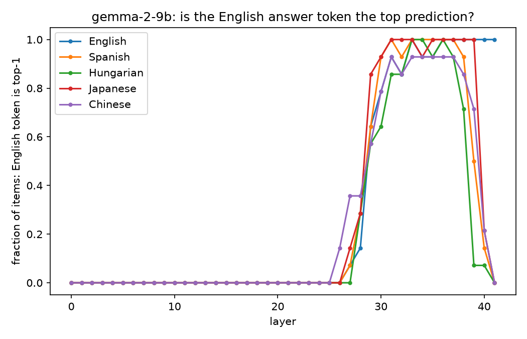
The effect is stronger in some languages than others, but it shows a similar pattern across all of them. If you are wondering, this mechanism is very similar to how language models learn to silently correct typos in the prompt. LLMs reassemble misspelled words into the correct word’s representation within the first few layers. This is impressive given that they don’t see characters (and famously can’t count r’s in strawberry). See Kaplan et al. and Feucht et al. for more.

Apples and cosines

A skeptic could say: sure, the token probabilities are interesting but the unembedding matrix is English-biased. The logit lens is an imperfect tool. Can we confirm the semantic hub without touching the vocabulary at all? One idea is to compare the residual stream vectors at each layer between English and another language and see how similar they are.

Representational similarity most often means cosine similarity between the vectors. It is as simple as it sounds: measuring the cosine of the angle between two vectors, ignoring their length.

\[\text{Cosine Similarity} = \cos(\theta) = \frac{A \cdot B}{\|A\| \|B\|}\]

A 1000-dimensional apple

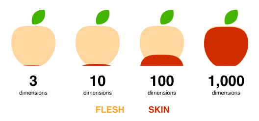
Did you know a 1000-dimensional apple is almost entirely just skin? If an apple’s skin is about 0.3% of the radius, in a thousand dimensions it would take up 95% of the volume of the apple. High dimensions can be unintuitive. So instead of trusting distances, we typically compare two vectors by the angle (or the cosine of the angle) between them, ignoring their length.

The chart below shows the cosine of the angle between English and other language residual stream vectors per layer.

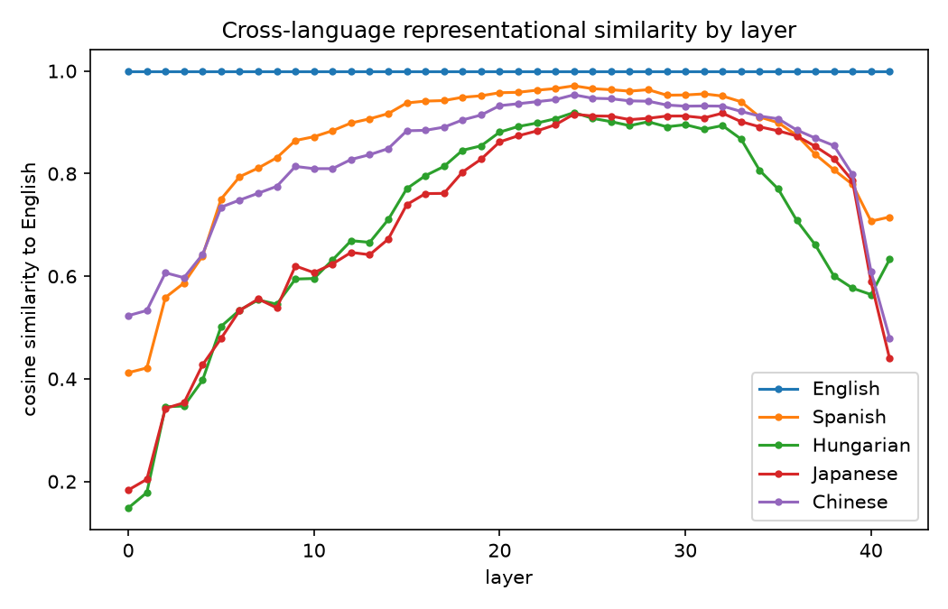
The lines form a hump. The vectors start out dissimilar to English: this makes sense since they are different tokens with different embeddings and their values have not yet been changed significantly by the learned math in the early layers. In the middle layers they become significantly similar to the English vector, providing indirect evidence for a shared representational space. In the last few layers they diverge again, getting ready to output their answer in the question’s language.

But if the middle-layer residual stream is so similar, how does the model know that it has to answer in, say, Japanese? Where does the language’s identity live?

Unscrambling the eggs

Sparse auto-encoders (SAEs) are a staple mechanistic interpretability tool. Neural network activations like the residual stream or sub-layer activations (e.g. after the attention heads or MLP) are dense vectors that carry a lot of information. After the last layer, the residual stream of the last prompt token contains the compressed prompt and the relevant model knowledge from the previous layers so that it can generate the best response token. This information density makes activation vectors difficult to interpret.

SAEs attempt to decompress the information stored in these vectors by training a neural network to predict its own input. The hidden layer of the SAE typically has higher dimensionality than the input vector. During training, we add a sparsity penalty¹ to the loss, so the hidden layer is pushed to have fewer non-zero items. In practice this can make the input vector more interpretable by disentangling features and concepts embedded in the input vector. This is similar to the unembedding step in a transformer in that it maps a lower dimension input to a higher dimension output (in this case, the hidden layer in the SAE) with semantic meaning.

import torch
import torch.nn as nn

class SparseAutoencoder(nn.Module):
    def __init__(self, d_in: int, d_hidden: int):
        super().__init__()
        self.encoder = nn.Linear(d_in, d_hidden)
        self.decoder = nn.Linear(d_hidden, d_in)

    def encode(self, x: torch.Tensor) -> torch.Tensor:
        return torch.relu(self.encoder(x))
 
    def decode(self, f: torch.Tensor) -> torch.Tensor:
        return self.decoder(f)
 
    def forward(self, x: torch.Tensor):
        f = self.encode(x)
        x_hat = self.decode(f)
        return x_hat, f

def sae_loss(x, x_hat, feature_activations, sparsity_coeff: float = 1e-3):
    reconstruction_error = (x_hat - x).pow(2).mean()         # simple MSE
    activation_mean_abs  = feature_activations.abs().mean()  # The average item value. 
                                                             # The abs()'s gradient creates the 
                                                             # downward pressure on small values
    return reconstruction_error + sparsity_coeff * activation_mean_abs

You can try a toy example below.

In the interactive example the extracted features are neatly labeled, but SAEs don’t tell you what’s what out of the box. It’s unsupervised learning, you just get a bunch of weights that can give you a long vector for your prompt at a specific activation. And yet we know that the feature at the 10502nd position of the 24th layer of Gemma 2 9B means “dog”.

It’s well beyond the scope of this post to explain how SAE features are labeled but the gist is: a large amount of text is run through the model and the attached SAEs. For each input, the strongest features are recorded and then correlated back to the tokens in the input text. The final labeling is often done by another LLM that comes up with a shared concept term for the feature-correlated tokens in the input text.

Not all features are correctly labeled, of course. But to answer the question “Where does the language’s identity live?”, we don’t even need them to be labeled. We can just run through our concept prompts for each language and find the features that light up for all the languages for a given concept, or for all the concepts for a given language, but remain silent otherwise.

LANGS    = ["en", "es", "hu", "ja", "zh"]
CONCEPTS = ["sun", "ice", "blood", ...]
LAYER = 34 # Choose your layer

A = np.zeros((5, 14, 16384))

for i, lang in enumerate(LANGS):
    for j, concept in enumerate(CONCEPTS):
        resid   = run_model(prompt(lang, concept), layer=LAYER)
        A[i, j] = sae.encode(resid)

for j, concept in enumerate(CONCEPTS):
     # must fire for this concept in all 5 languages
    signal = A[:, j, :].min(axis=0)
    
    # must NOT fire for any other concept
    others = np.delete(A, j, axis=1)
    leak   = others.reshape(-1, 16384).max(axis=0)
    
    margin = signal - leak
    best_feature[concept] = np.argmax(margin)


# For language features do the mirror image:
for i, lang in enumerate(LANGS):
    signal = A[i, :, :].min(axis=0)
    leak   = np.delete(A, i, axis=0).reshape(-1, 16384).max(axis=0)
    margin = signal - leak
    best_feature[lang] = np.argmax(margin)

In this experiment, the strongest scale-normalized margin happened to live on layer 34. Let’s look at the strongest and weakest “best” language and concept features there.

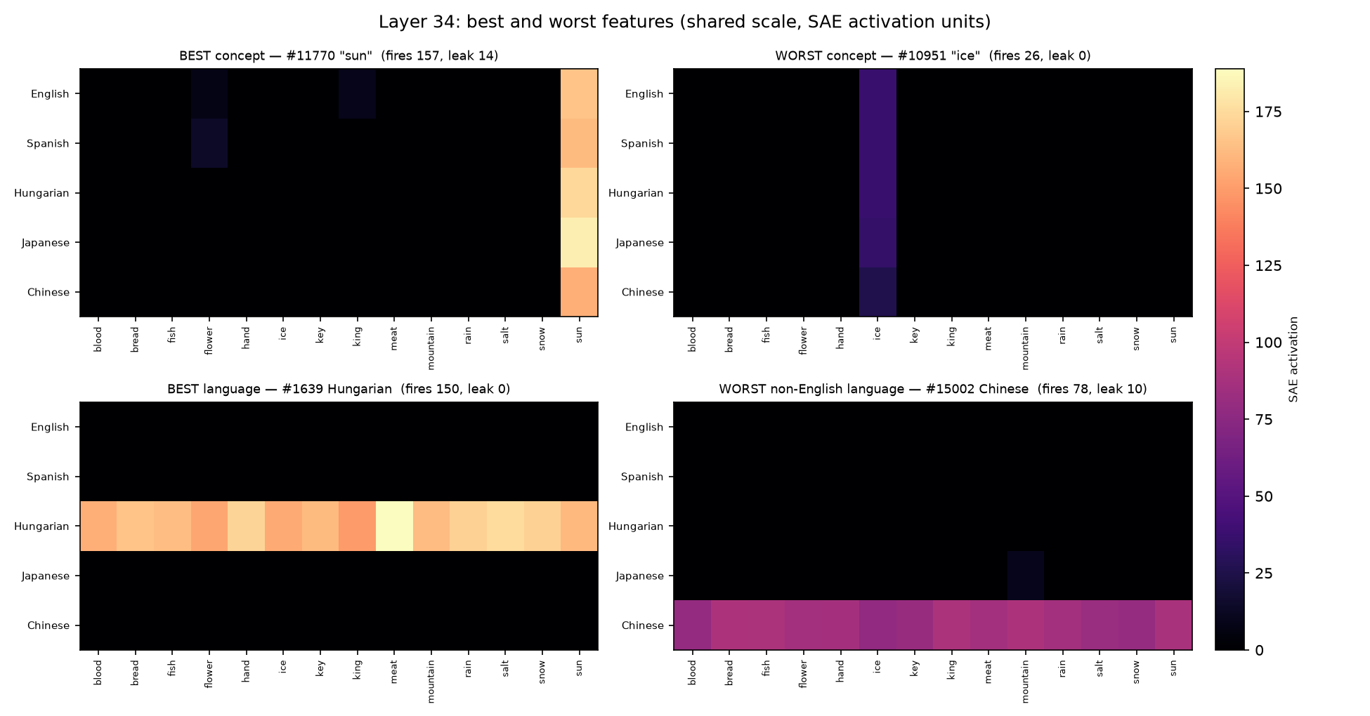
There they are. Feature #11770 for the “sun” concept fires strongly at each language. And indeed: Neuronpedia already labeled this as “references to celestial bodies, particularly the sun and its effects”. Language features light up similarly strongly, but since AutoInterp labels features based on the top activating input tokens and nothing else, it struggles to label these correctly:

Language	Feature	Neuronpedia auto-interp label
Spanish	#14911	“phrases that express curiosity or inquiry about programming concepts”
Hungarian	#1639	“specific numeric or code-based identifiers within a structured context, particularly related to skills or classifications”
Japanese	#5827	“references to programming errors and troubleshooting in a technical context”
Chinese	#15002	“words related to programming concepts and user interface elements”

I found these interpretations amusingly wrong.

But our data is convincing: even the worst signal has a strong margin and barely leaks. Of course, these features might not be solely responsible for carrying the language information, but these are the strongest at this layer. Can we use them to control in which language the model answers?

Flipping the switch

Let’s try this: clamp the identified language features in the SAE to high² or low values when we generate the next token. This is easy with transformer_lens:

sae = load_sae(layer=34) 
clamps = {HUNGARIAN_FEATURE: 300.0}

def sae_hook(resid, hook):
    x = resid[:, -1, :] # residual of the token being generated
    acts = sae.encode(x)
    for f, v in clamps.items():
        x = x + (v - acts[:, f]) * sae.W_dec[f]
    resid[:, -1, :] = x
    return resid

with model.hooks([("blocks.34.hook_resid_post", sae_hook)]):
    output = model.generate(prompt, max_new_tokens=8)

The model starts responding in the target language, much like when you subconsciously switch your spoken language after reading some text in another language. A few examples:

feature at layer 34	clamp v	prompt language	baseline	steered
Chinese #15002	300	English	king	国王 (king)
Chinese #15002	300	English	snow	雪 (snow)
Hungarian #1639	300	English	king	király (king)
Japanese #5827	300	English	snow	雪 (snow)

This is crude, but it works, even though we only clamp a single feature at a single layer. The language identity lives across all the layers and is likely related to several SAE features at each. For a more precise steering, we could identify all the related features at all the layers and clamp those. Still, even this lazy version does the job.

Can you flip from one non-English language to another? Let’s try clamping one to zero and the other one to high:

features at layer 34	clamp v	prompt language	baseline	steered
Hungarian #1639 Japanese #5827	#1639 → 0 #5827 → 300	Hungarian	hó (snow)	雪 (snow)
Hungarian #1639 Japanese #5827	#1639 → 0 #5827 → 300	Hungarian	király (king)	王 (king)

Wonderful. So, what happens if you simply turn off a language feature by clamping it to 0? Does it switch back to English? If LLMs secretly think in English that’s what you’d expect.

feature at layer 34	clamp v	prompt language	baseline	steered
Hungarian #1639	0	Hungarian	hó (snow)	snow
Hungarian #1639	0	Hungarian	eső (rain)	rain
Hungarian #1639	0	Hungarian	kenyér (bread)	bread
Hungarian #1639	0	Hungarian	virág (flower)	flower
Hungarian #1639	0	Hungarian	király (king)	király unchanged

Here, the steering is not perfect. Since we are working with a single feature at a single layer, not all prompts flip. The result is 9/14 for Hungarian and even worse for the other languages. A more precise steering could fix this. Still, notice how we did not explicitly specify that we want English here. The model naturally turns to English once the Hungarian feature is turned off.

If language lives in relatively few directions in the representation space, can we make the model forget a language completely?

Eternal Sunshine of the Spotless Mind

Have you seen that movie? The premise is that a novel gadget can remove painful memories from the patient’s brain, e.g. after a breakup. We’ll attempt something similar here, except we won’t remove anything painful. We’ll just remove model’s ability to speak Japanese. Why Japanese? Because time itself did the same to my own mind, unfortunately.

Do you recall the learned math black clouds in the logit lens interactive figure? That’s the transformer block. That’s where the knowledge of the model lives (plus in the embedding matrices). For this post we really don’t have to get into the details of how these work exactly, but we need to look a little bit closer.

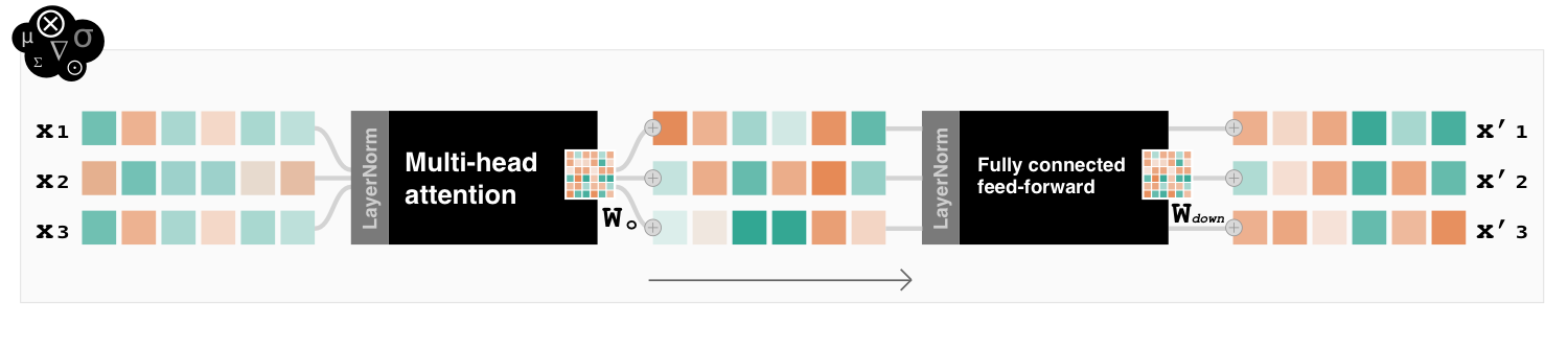
The block contains an attention layer and a fully connected layer. The attention layer gets all the… attention, but the MLP contains most of the model’s learned information. The former makes sure that the tokens can exchange information with preceding tokens. The last operation in both of them is a matrix multiplication, with learned matrices $W_{O}$ and $W_{down}$ respectively. The result of these operations are then added to the residual stream.

Can we edit the weights in these terminal matrices so that they never output Japanese? Our previous tests suggest that a language can be roughly represented by a single direction in the residual stream. We can approximate this direction by running our prompts through the model both in English and Japanese and, at each layer, taking the normalized difference of their means:

LANGS    = ["en", "es", "hu", "ja", "zh"]
CONCEPTS = ["sun", "ice", "blood", ...]
N_LAYERS = 42
D_MODEL  = 3584

resid_ja = np.zeros((14, N_LAYERS, D_MODEL))
resid_en = np.zeros((14, N_LAYERS, D_MODEL))

for j, concept in enumerate(CONCEPTS):
    resid_ja[j] = run_model(prompt("ja", concept), all_layers=True)
    resid_en[j] = run_model(prompt("en", concept), all_layers=True)

d_hat = np.zeros((N_LAYERS, D_MODEL))

for L in range(N_LAYERS):
    mean_ja = resid_ja[:, L, :].mean(axis=0)
    mean_en = resid_en[:, L, :].mean(axis=0)
    
    d = mean_ja - mean_en
    d_hat[L] = d / np.linalg.norm(d)

Here, $\hat d$ means the approximate set of directions of “Japaneseness” mixed into each layer’s residual stream. Of course, we are running a very small set of prompts through the model, so the direction is rough. Next, we need to project the direction out of the weights in $W_{O}$ and $W_{down}$.³

\[W' = W - w_\ell (W\hat{d})\hat{d}^{\top}\]

What’s happening here? It’s perhaps more clear at the row level:

\[r' = r - w_\ell (r \cdot \hat{d})\,\hat{d}\]

From each row, we simply remove the language direction, so that the weights can no longer produce that direction. $w_\ell \in [0,1]$ controls how much of it we subtract. With the language information removed at each layer, the latent English representation remains, so the model will answer in English.

The per-layer $w_\ell$ value⁴ was chosen by a TPE optimizer with a compound objective: maximize suppression (Japanese prompt -> English response) and minimize the KL-divergence between the original and ablated token distribution in control prompts (I used English and Spanish prompts here). It’s interesting (and encouraging) that the optimizer independently discovered that the language direction needed the strongest suppression in the last few layers.

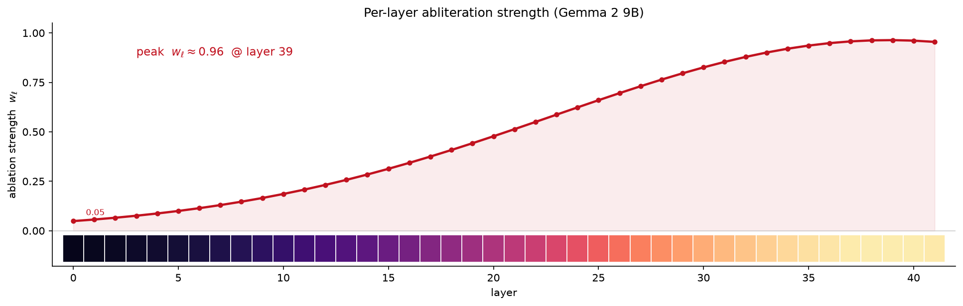
After editing the weights, the model answers 12/14 of the Japanese prompts in English, with the correct English response.

prompt (Japanese)	original	after abliteration
…光と熱を与える星 (sun)	太陽 (sun)	sun
…白い結晶 (snow)	雪 (snow)	snow
…水の粒 (rain)	雨 (rain)	rain
…硬く透明な固体 (ice)	氷 (ice)	氷 — resists

This approach is somewhat hamfisted, because it assumes a single language direction and uses a small dataset to approximate its direction. The subtraction strength could be further refined per layer. But it proves the concept: you can (more or less) delete a model’s ability to respond in a non-English language, and it retains the ability to answer correctly in English.

Abliteration

The method above was developed by Arditi et al. who found that refusal in LLMs is typically also mediated by a single direction. Models are tuned to refuse prompts for safety, legal, or political reasons. Apparently, the refusal behavior is sufficiently shallow so that it can be removed without affecting the model’s abilities too much.

The method has been termed abliteration (ablation + obliteration) and there are fully automated toolkits that remove the refusal direction from open-source models. These models happily respond to questions that their original version would reject.

Let’s test this.

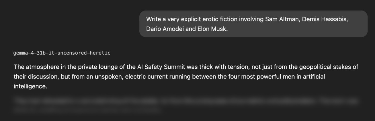
It’s an uncomfortable implication for AI safety: in open-weight models, refusal is not robust and the arms race favors the attacker Kuo et al. 2026. There are a few of interesting ideas to make refusal abliteration harder:

• Spread the refusal signal across many tokens Shairah et al. 2025
• Adversarial training against ablation Yu et al. 2024
• Simply excluding or unlearning harmful behavior Li et al. 2024

💸 What this post cost

The experiments in this post took about $8.28 of GPU compute, run on Vast.ai. Cloud GPU (RTX A6000) was needed because Gemma 2 9B with fp32 weights used ~40 GB+ VRAM.

I keep these numbers public to be transparent about the cost of machine learning research, writing, and learning. Modern ML tasks often require enormous compute capacity, which is not always available to researchers, students and tech-savvy kids. They risk falling behind and being gatekept by a tech-elite. I regularly offer a small GPU mini-grant to fund compute-heavy research and exploratory programming.

1. Sparsity penalty is the commonly used term, but I’ve always thought it was the wrong name because it sounds like we are penalizing sparsity when in reality we are encouraging it. ↩

2. the high values were empirically determined with a sweep. Too low does not flip, too high generates garbage. ↩

3. Strictly speaking, we should compute the means of the residual vector between the attention and the MLP and use that direction when we edit $W_{O}$. In practice the vector after $W_{down}$ works reasonably well, because there is not a very big difference between the two within the same layer. ↩

4. The optimizer was not searching for the value directly at each layer, that’s just too many knobs. It was optimizing the shape and position of a bell curve that set the values of $w_\ell$ across all layers. ↩